How to Freeze Panes in Excel
Freezing panes in Excel is an essential feature that allows users to keep specific rows or columns visible while scrolling through the rest of the worksheet. This functionality is particularly useful for managing large datasets, where headers or labels need to remain in view for better context and readability. In this comprehensive guide, we will delve deep into the various aspects of freezing panes in Excel, including step-by-step instructions, practical examples, troubleshooting common issues, and best practices.
Table of Contents
- Introduction to Freezing Panes
- Importance of Freezing Panes
- How to Freeze Panes
- Freezing Top Row
- Freezing First Column
- Freezing Multiple Rows and Columns
- Practical Examples of Freezing Panes
- Freezing Header Rows
- Freezing Side Labels
- Combining Frozen Rows and Columns
- Advanced Techniques
- Dynamic Freezing Based on Data
- Using Named Ranges with Frozen Panes
- Troubleshooting Common Issues
- Unfreezing Panes
- Issues with Split Panes
- Handling Large Datasets
- Best Practices for Freezing Panes
- When to Use Freezing Panes
- Alternatives to Freezing Panes
- Optimizing Performance
- Conclusion
1. Introduction to Freezing Panes
Freezing panes in Excel is a feature designed to help users keep specific parts of their worksheet visible while scrolling through other sections. This is achieved by locking rows or columns in place, ensuring that critical information such as headers or labels remains on-screen at all times.
What is Freezing Panes?
Freezing panes essentially locks certain rows or columns in place. For example, if you freeze the top row, it will always be visible even as you scroll down through hundreds of rows of data. Similarly, freezing the first column ensures that it remains visible as you scroll horizontally.
2. Importance of Freezing Panes
Freezing panes is crucial for improving the usability of Excel worksheets, especially when dealing with large datasets. Here are some reasons why freezing panes is important:
- Enhanced Readability: Keeps headers or labels visible, making it easier to understand the data context.
- Efficient Navigation: Allows users to navigate large datasets without losing track of key information.
- Improved Data Entry: Facilitates data entry by keeping important reference points in view.
- Better Presentations: Makes it easier to present data to others without constant scrolling.
3. How to Freeze Panes
Excel provides several options for freezing panes. Depending on your needs, you can freeze the top row, the first column, or multiple rows and columns simultaneously.
Freezing Top Row
Freezing the top row is useful when your dataset has column headers that you need to keep visible.
Steps to Freeze Top Row:
- Open your Excel worksheet.
- Go to the View tab on the Ribbon.
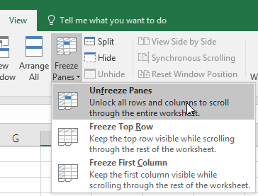
- Click on the Freeze Panes dropdown.
- Select Freeze Top Row.
Example:
If your worksheet has column headers in row 1, freezing the top row will ensure these headers remain visible as you scroll down through the data.
Freezing First Column
Freezing the first column is useful for keeping row labels or identifiers visible while scrolling horizontally.
Steps to Freeze First Column:
- Open your Excel worksheet.
- Go to the View tab on the Ribbon.
- Click on the Freeze Panes dropdown.
- Select Freeze First Column.
Example:
If your worksheet has row labels in column A, freezing the first column will keep these labels visible as you scroll to the right.
Freezing Multiple Rows and Columns
To freeze multiple rows and columns, you need to select a cell that is below the rows and to the right of the columns you want to freeze.
Steps to Freeze Multiple Rows and Columns:
- Select the cell just below the rows and to the right of the columns you want to freeze.
- Go to the View tab on the Ribbon.
- Click on the Freeze Panes dropdown.
- Select Freeze Panes.
Example:
To freeze the first two rows and the first two columns, select cell C3 before choosing the Freeze Panes option.
4. Practical Examples of Freezing Panes
Understanding how to apply freezing panes in practical scenarios can help you manage your data more effectively.
Freezing Header Rows
Scenario:
You have a large dataset with headers in the first row.
Steps:
- Go to the View tab.
- Click Freeze Panes.
- Select Freeze Top Row.
This ensures that your headers remain visible as you scroll down through the data.
Freezing Side Labels
Scenario:
Your worksheet has row labels or identifiers in the first column.
Steps:
- Go to the View tab.
- Click Freeze Panes.
- Select Freeze First Column.
This keeps your row labels visible while you scroll horizontally.
Combining Frozen Rows and Columns
Scenario:
You need both the top row and the first column to stay visible.
Steps:
- Select the cell just below the top row and to the right of the first column (typically B2).
- Go to the View tab.
- Click Freeze Panes.
- Select Freeze Panes.
This will freeze the first row and the first column simultaneously.
5. Advanced Techniques
For more complex data management tasks, advanced freezing techniques can be employed.
Dynamic Freezing Based on Data
Scenario:
You want to freeze panes dynamically based on the presence of certain data.
Steps:
- Use VBA (Visual Basic for Applications) to create a macro that automatically freezes panes based on specific criteria.
- Write a macro that identifies the data range and applies the Freeze Panes command accordingly.
Example VBA Code:
Sub DynamicFreezePanes()
 Dim ws As Worksheet
 Set ws = ActiveSheet ' Identify the row and column to freeze
 Dim freezeRow As Integer
 Dim freezeCol As Integer
 freezeRow = 2
 freezeCol = 2 ' Apply Freeze Panes
 ws.Cells(freezeRow, freezeCol).Select
 ActiveWindow.FreezePanes = True
 End Sub
Using Named Ranges with Frozen Panes
Scenario:
You have specific named ranges that you want to keep visible.
Steps:
- Define named ranges for the rows or columns you want to freeze.
- Use the Freeze Panes feature in conjunction with the named ranges to keep the relevant data in view.
Example:
Define a named range for the header row and another for the first column. Then use these ranges to set up your freezing points.
6. Troubleshooting Common Issues
Freezing panes can sometimes lead to issues. Here are some common problems and their solutions.
Unfreezing Panes
Problem:
You no longer need the panes to be frozen.
Solution:
- Go to the View tab.
- Click on the Freeze Panes dropdown.
- Select Unfreeze Panes.
Issues with Split Panes
Problem:
Accidentally splitting panes instead of freezing them.
Solution:
- Ensure you select the correct cell before freezing panes.
- If panes are split, go to the View tab and select Remove Split before applying Freeze Panes.
Handling Large Datasets
Problem:
Excel slows down when freezing panes in large datasets.
Solution:
- Optimize your dataset by removing unnecessary data or calculations.
- Consider breaking down large datasets into smaller, more manageable worksheets.
7. Best Practices for Freezing Panes
Following best practices can help you effectively use the Freeze Panes feature without compromising the functionality of your worksheet.
When to Use Freezing Panes
- Consistent Headers: Use freezing panes when you need to keep headers visible at all times.
- Row Labels: Freeze panes to keep row labels in view for easy reference.
- Complex Navigation: Apply freezing panes for complex datasets that require constant reference to certain rows or columns.
Alternatives to Freezing Panes
- Split Panes: For scenarios where you need to view different parts of the worksheet simultaneously, consider using Split Panes.
- Tables: Convert your data into an Excel table to leverage built-in filtering and header visibility features.
Optimizing Performance
- Limit Freezing: Only freeze the rows or columns you need to keep visible.
- Data Management: Regularly clean and optimize your dataset to maintain performance.
8. Conclusion
Freezing panes in Excel is a powerful feature that enhances the usability and readability of large datasets. By keeping specific rows or columns visible, you can maintain context and improve data entry, analysis, and presentation. Understanding how to effectively use and troubleshoot this feature will significantly improve your Excel skills and efficiency.
By following the detailed steps, practical examples, and best practices outlined in this article, you can master the Freeze Panes feature and apply it effectively to your data management tasks. Whether you are a beginner or an advanced user, these insights will help you optimize your use of Excel and manage your data more effectively.